Analyze experiment data

Find the direct beam position

In experiments, the detector may not be mounted on a diffractometer rotation arm and move in a circular track. In such case, the “Find direct beam” function based on the “detector location” will not work. If the detector position is accurately surveyed, the direct beam position can be manually calculated from geometry of the beam-sample-detector triangle; otherwise, the “Find direct beam” function based on “Diffraction pattern” will help to estimate direct beam X and Y. Basically, users will be asked to mark out a diffraction ring and provide information about the d-spacing of the atomic plane and the harmonic energy that this ring is generated with. In practice, a simple and high-quality diffraction pattern from a reference sample should be used to facilitate the locating of direct beam position. Below is the detailed procedure:

1. Input experiment parameters and the sample structure. In this example, a transmission-mode diffraction pattern from Al foil was used.
2. Load the diffraction pattern. If the raw data is multi-frame tiff file, the program will calculate the mean intensity of each frame and plots them in a figure. A dialog window will pop up simultaneously, asking which frame to load.

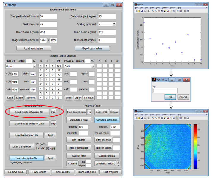
Figure 11: Load diffraction data

3. Load the energy spectrum.
4. In the space to the right of the “Find direct beam” button, input the number of times that this process will be repeated. Users may choose to calculate direct beam X and Y for multiple times based on one specific diffraction ring to increase statistical accuracy, or based on different rings as long as the d-spacings and harmonic energies are known for these rings.
5. Click “Find direct beam” button and choose “Diffraction pattern”. A message window will show up with the instruction for this process. Read it carefully, and click “OK” to proceed. The diffraction pattern that was loaded will then appear.
6. On the diffraction pattern, use three points to define the diffraction ring. Single-click the first two points, and double-click the last one to complete the marking. Once confirmed, a dialog window will pop up asking the energy and d-spacing associated with this diffraction ring. Click “OK” to proceed.
7. If users choose to do multiple times, repeat step (6) until it all finishes.
8. The program will do the calculation and the direct beam X and Y values will show up in the GUI control panel.

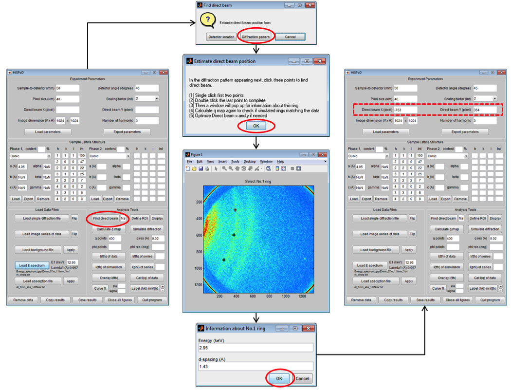
Figure 12: Procedure to estimate direct beam position based on a diffraction pattern

9. Click “Calculate q map” to verify the direct beam position. Note that “q res (A)” has to have a number for this function. A figure with three panels will pop up. The left image is the q map corresponding to the selected 1^st harmonic energy. The middle panel shows the map of azimuthal phi angles. The right image is the diffraction pattern overlaid with reference diffraction peaks (again corresponding to selected 1^st harmonic energy). If the reference peak positions deviate much from the diffraction rings. Repeat the whole process and make sure the input of the diffraction ring information is correct. Note that those peaks which are generated by the n^th harmonic energies (n>1) are not labeled here.

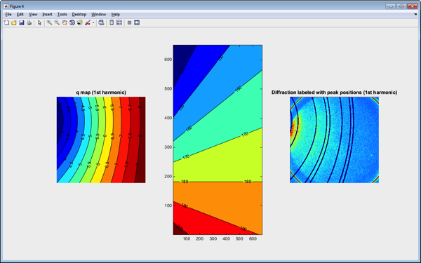
Figure 13: Calculate q and phi maps to verify the direct beam position

10. To more accurately locate the direct beam position, click “Label (hkl) in I(tth)” button, and choose “Experiment”. The I(tth) plot will show up with diffraction peaks labeled. Slightly adjust the direct beam position and repeat this process until the peak positions in the data match the reference. Note that each time the direct beam X and Y are changed, q map has to be calculated before using the labeling I(tth) function.

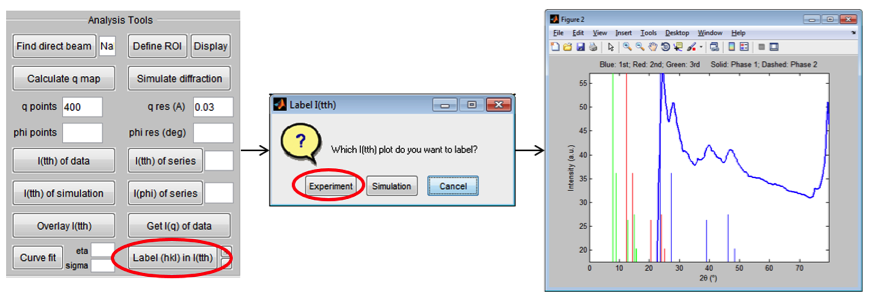
Figure 14: Fine optimize the direct beam position

11. Verify the direct beam position and the other experiment parameters by analyzing data from different reference samples, different detector angles, or different undulator gaps. The results should be consistently reasonable.

Procedure for analyzing diffraction patterns

Once the accurate direct beam X and Y are obtained, the program is ready to analyze user experiment data. Actually, most of the functions to be used have been mentioned above. A typical procedure is described below.

Calculate I(tth) of individual diffraction pattern

1. Input or load sample structure.
2. Load diffraction data.
3. Load energy spectrum.
4. Load and apply the absorption file if the transmission geometry is used. (Optional)
5. Click “Define ROI” to mark out the region of interest. A message window will show up providing two options for ROI defining. Click “Full frame” is no region in intended to be masked out; click “Click to define” for selecting a certain region. Then, another message window will show up with detailed instructions. Click “OK” to proceed.
6. In the diffraction pattern popping up, single-click the mouse left button at multiple spots (unlimited number) to define the region to be analyzed. Overlap the last the spot with the first one to complete the marking. Double-click the selected area to confirm. Once defined, the program will remember the ROI and automatically apply to the new data loaded. To analyze data with different ROI, simply re-define it.

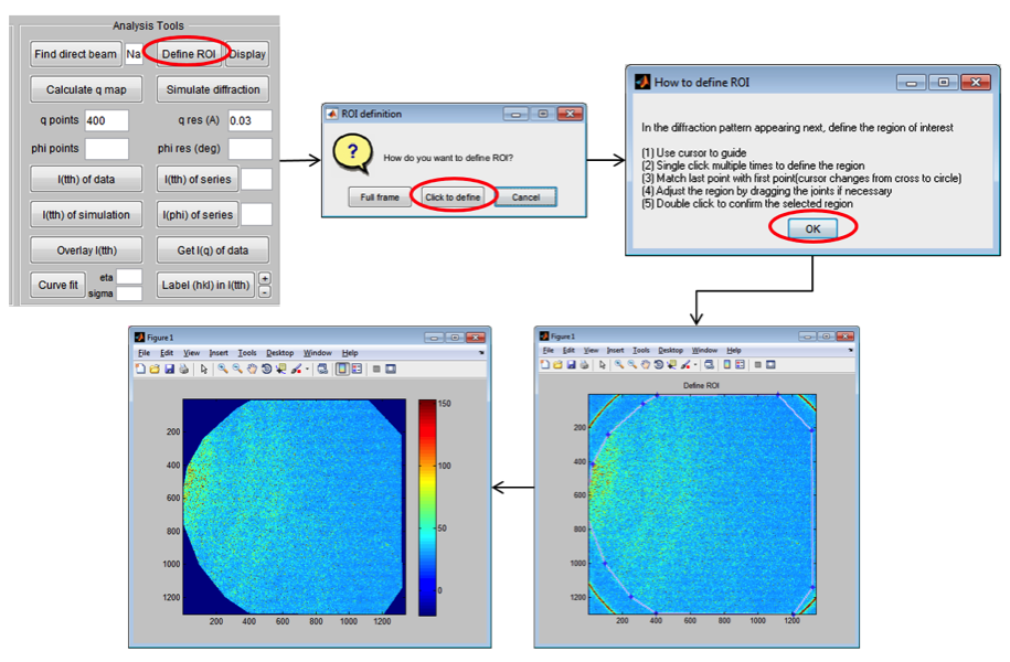
Figure 15: Define the region of interest

7. Click “Calculate q map”. The diffraction rings should overlap with the reference peak positions perfectly.

8. Click “I(tth) of data” button. A dialog window will pop up, asking “Do you want to perform the radial averaging over all angles or a certain range of angles?” This is useful when dealing with diffraction anisotropy, such as the cases of tensile or compressive loading. If choose “All”, the program will integrate all pixels within ROI. If choose “Segment”, another window will pop up, asking whether you need to input the starting and ending azimuthal angles or click in the diffraction pattern to define the angle range. Choose “Input” to type in the angles in the following pop-up window; or choose “click” and then single click the starting angle, and double click to select the ending angle.

   

   

   

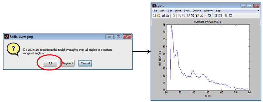
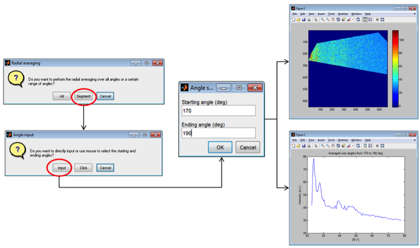
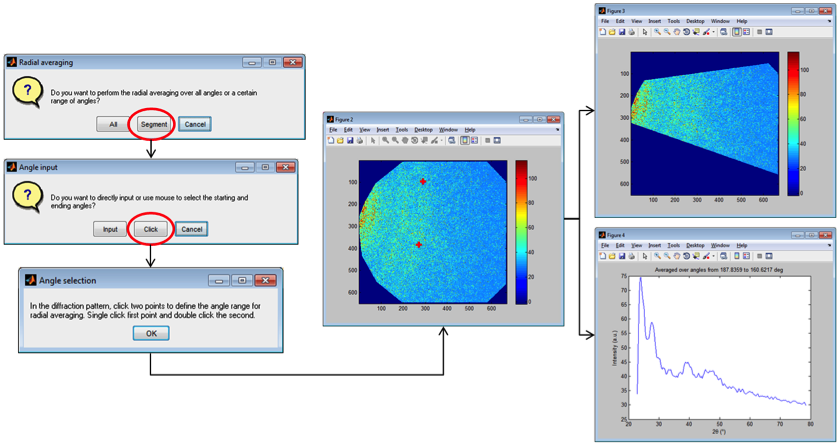
   Figure 16: Calculate 1D intensity profile

9. Click “Label (hkl) in I(tth)” button and choose “Experiment” to index the diffraction plot. Click “+” and “-” buttons to adjust the relative heights of the reference bars.

10. Click “Get I(q) of data” button to get 1D intensity as a function of the reciprocal wavevector. (Optional) Here the q is calculated with the 1^st harmonic energy.

Calculate I(tth) of a series of diffraction patterns

1. Input or load experiment parameters, sample structure, energy spectrum, and absorption data as routine.

2. Load data series by clicking “Load diffraction data series” button. A directory window will pop up asking for data selection. Choose files to be analyzed, and click “Open” to load them. The first pattern in the series will be displayed.

   

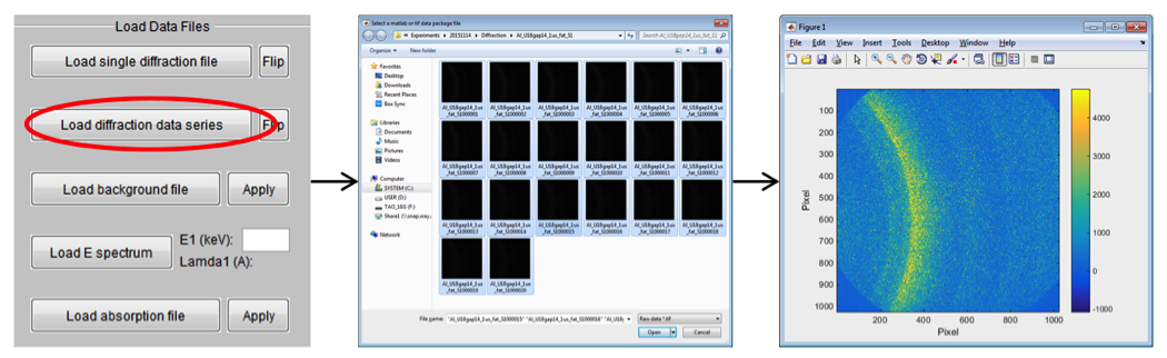
   Figure 17: Load data series

3. Calculate q map and define ROI as routine.

4. Click “I(tth) of series” button to obtain 1D intensity profiles from the loaded data files. The space to the right of the button takes input of a number, which will help spacing individual intensity profile off in the final plot, as shown in Fig. 18. Once clicked, a message window will show up with the instruction for the following step. Click “OK”, then a 2D intensity pattern will show up. The vertical axis is the frame number, and the horizontal axis is 2theta scattering angle. This is a pattern that piles all individual 1D intensity profiles together, which helps the user to observe the change in the scattering intensity due to a certain sample event. Click two points laterally (i.e. within same frame) in a flat part of the intensity map to define an angle range that contains flat background. Then all 1D intensity profiles will subtract their own background intensity (calculated within the same angle range), and re-pack together to generate a new 2D intensity pattern. Along with background subtraction, the new 2D intensity pattern will be populated in pixels via data interpolation, in order to display a smoother visualization effect.

5. Similar to the analysis of individual diffraction pattern, one can choose to perform radial integration over all available azimuthal angles or a certain angle range.

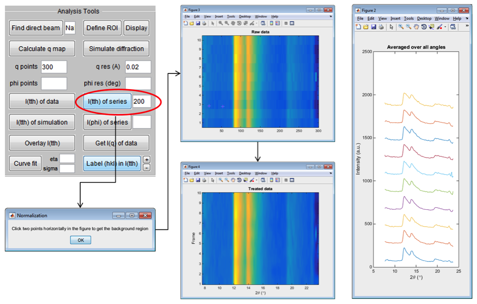
Figure 18 Calculate 1D intensity profiles for a batch of diffraction patterns

Calculate I(phi)