Appendix

Diffraction simulation

The simulation of a white-beam diffraction pattern from a known material starts from the calculation of monochromatic beam diffraction patterns for the specific detector location, I(θ,E). Then these mono-beam diffraction patterns are integrated over the entire energy range with weighting factor being the flux of photons with different energy, F(E).

\[I_{white} = \int_{E_{1}}^{E_{2}} I(\theta,E) \cdot F(E)\,dE.\]

where E₁ and E₂ are typically 1 keV and 60 keV, respectively. To improve the calculation speed, discrete diffraction peaks are considered, meaning that I(θ,E) is normally replaced by a series of I_hkl(θ,E). Equation above then becomes:

\[I_{white} = \int_{E_{1}}^{E_{2}} \left(\displaystyle\sum_{i=1}^{n} I_{hkl_{i}}(\theta,E)\right) \cdot F(E)\,dE.\]

In our simulations, the diffraction peak shape is described using the pseudo-Voigt function:

\[V(x) = \left(\frac{1-\eta}{\sigma\sqrt{2\pi}}\right) \cdot exp\left({\frac{x^2}{2\sigma^2}}\right) + \eta \cdot \frac{\sigma}{2\pi} \cdot \frac{1}{x^2 + \left(\frac{\sigma}{2}\right)^2}\]

Essentially, the white-beam diffraction intensity at a given scattering angle is the convolution of the input diffraction intensity of different atomic planes with the energy spectrum of the x-rays.

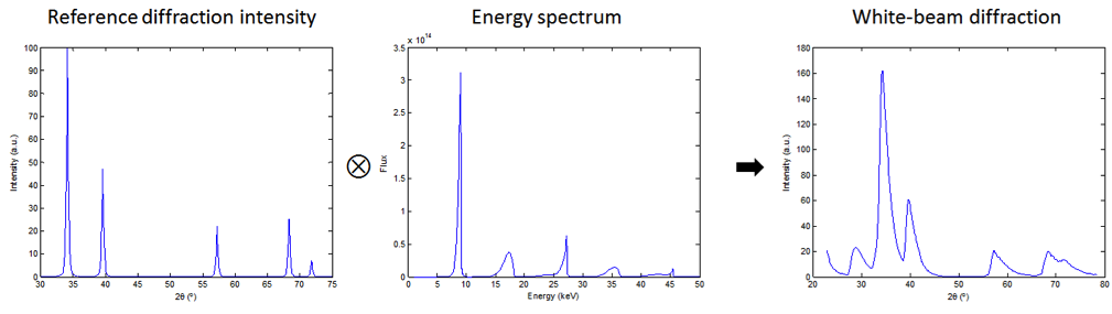
Figure 23: Simulation of white-beam diffraction

How to obtain the sample absorption file

Option 1: Ask the beamline scientists for it. If users are not confident to calculate the attenuation curve, asking the beamline scientists is always the best choice. Provide sample parameters including chemical formula, mass density, and thickness. For example, sample Al₂O₃, density of 3.95 g/cm³, thickness 500 µm.

Option 2: Use the web tool of The Center of X-Ray Optics. Calculate the x-ray transmission for a solid with procedure shown below and in Fig. 24.

• Fill in sample information
• Select energy range
• Click “Submit Request” to do the calculation. Another window will then pop up with the plot
• Click “data file here” to show the values
• Copy the data (without the sample info lines), and save it as a *.txt file

Note that this online tool can only calculate the transmission for energy ranging from 0-30 keV, which often not suffice for white-beam experiments.

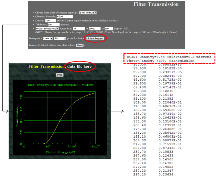
Figure 24: Calculate x-ray transmission at the website of CXRO

Option 3: Self calculate based on the x-ray mass attenuation coefficients from the NIST web page. There the attenuation coefficients (µ/ρ) are provided for elements from Hydrogen to Uranium. The x-ray attenuation T is calculated as:

\[T = exp\left({-\frac{\mu}{\rho}}\cdot \rho \cdot t \right)\]

where µ/ρ is value directly from the web page, ρ is the mass density of the sample, and t is the sample thickness.

For compounds, the attenuation coefficients will simply be the weighted-sum of each element:

\[\frac{\mu}{\rho} = \displaystyle\sum_{i} w_i \cdot \left(\frac{\mu}{\rho}\right)_i\]

where w_i is the weight (or mass) fraction of element i.

For example of Al₂O₃, density 3.95 g/cm³, thickness 500 µm, and for x-ray energy 10 keV, the mass coefficient of the sample will be:

\[\frac{\mu}{\rho} = \frac{27 \times 2}{27 \times 2 + 16 \times 3} \times 25.43 + \frac{16 \times 3}{27 \times 2 + 16 \times 3} \times 5.565 = 16.08 cm^2/g.\]

The attenuation will then be:

\[T = exp(-16.08 \times 3.95 \times 500 \times 10^{-4}) = 0.042\]

Some comparisons to guide the usage

1. Scaling factor: 4 vs 2 vs 1

   Always, the larger the scaling factor, the faster the processing time, yet the smaller the resolution. For the example shown in Fig. 25, the simulation time for scaling factor 4, 2, and 1 are 11 min, 1.5 min, and 14 sec, respectively. (Note the CPU is Intel i7, 3.4 GHz) Clearly, the small peak at 48° can only be visualized in the patterns with scaling factor 2 and 1. The effect of scaling factor on the analysis of experiment data is not as obvious, as the signal-to-noise ratio of single-pulse diffraction patterns is rather low and radially averaging is more related to the parameters “Points” and “Q res”. For image with dimension of about 1k x 1k, the scaling factor of 2 may be a good option.

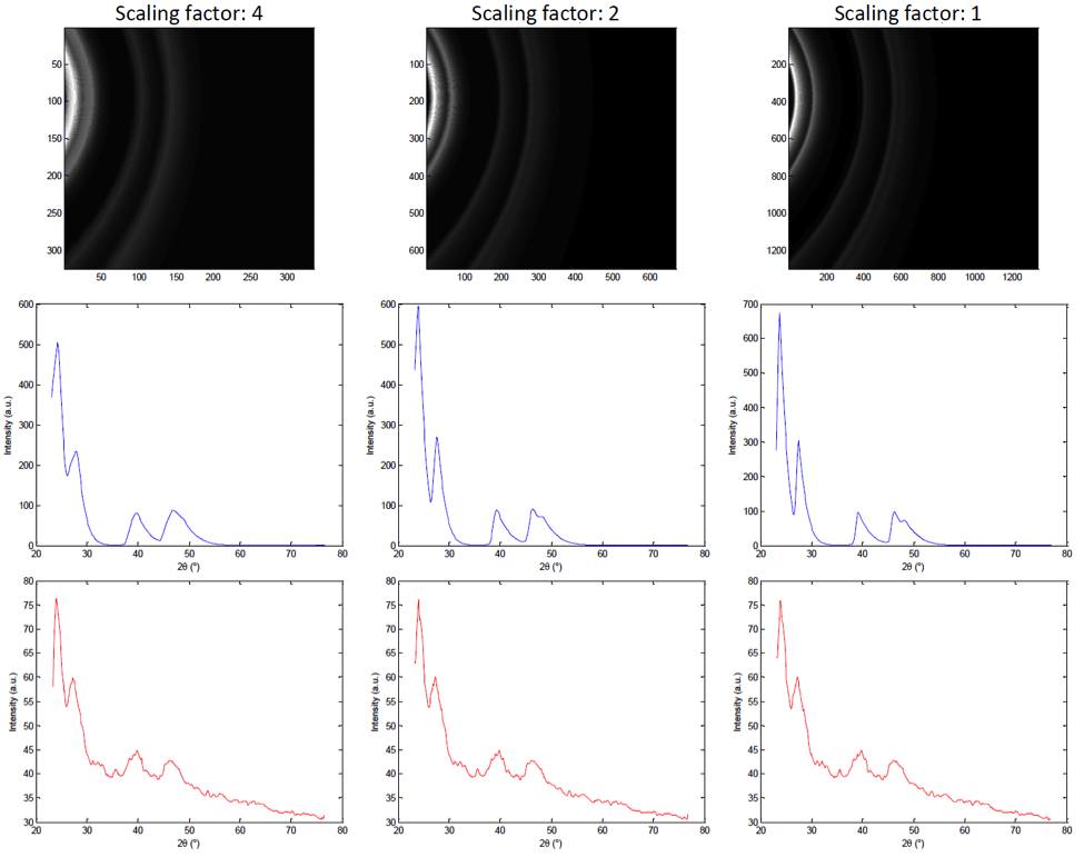
Figure 25: Effect of scaling factor

2. Direct beam position: wrong vs right

Figure 26 show the overlap of diffraction rings with the reference peaks in cases of wrong and correct direct beam position input. The correct parameters should satisfy all other data, either same sample with different undulator gap (i.e. energy spectrum) or other samples. For this specific example in Fig. 26, all the diffraction rings are generated by the 1^st harmonic energy, so they are all labeled, but this is not always the case. Figure 27 show the data from another undulator gap, in which some diffraction rings are generated by 2^nd harmonic energy. Users may simply input the photon energy used for labeling in the “E1 (keV)” space.

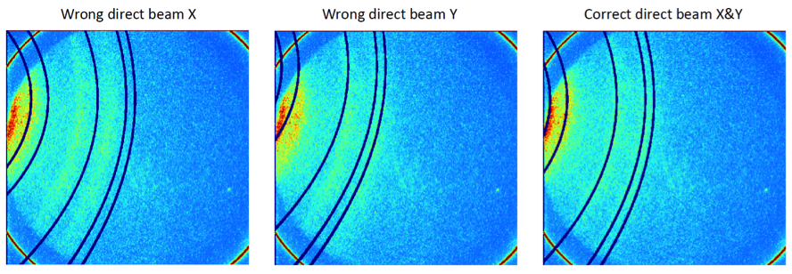
Figure 26: Effect of direction beam locating on calculation of q map

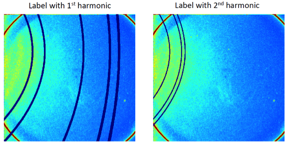
Figure 27: Reference peaks corresponds to 1st and 2nd harmonic energies

3. Pointes and Q res: rough vs smooth plots

Smooth plot looks good, but may lose some structure information due to the over averaging.

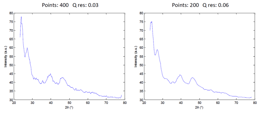
Figure 28: Rough and smooth (yet low-resolution) 1D plots

4. Region of interest: without ROI vs with ROI

This is not necessary if all the pixels on the detector function properly.

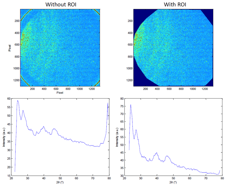
Figure 29: Effect of ROI on the 1D plot