Correlate simulation with experiment data
HiSPoD doesn’t have a function to automatically fit the 1D diffraction intensity profiles. The curve fitting function here is a direct overlay of the experiment data and simulated results. If strain information is desired, manually adjust the lattice parameter until the simulation matches the experiment data perfectly. A typical procedure to correlate the simulation with data is described below:
- Input or load experiment parameters and sample structure information.
- Load diffraction data, energy spectrum, and absorption file.
- Define ROI, and Calculate q map.
- Get I(tth) of data.
- Simulate “Realistic” diffraction pattern.
- Get I(tth) of simulation.
- Click “Overlay I(tth)” button in the “Tools” module. A message window will pop up telling users to get the noise level. Click “OK” to proceed. In the diffraction pattern, circle out a region (typically at the detector corners that are outside the scintillator) to collect the mean detector noise, and double-click to confirm. Another message window will pop up with instructions on how to define the background. Click “OK” to proceed. The 1D intensity profile of the experiment data will show up, in which multiple points need to be selected to define the background. Here the background (i.e. combination of the tail part of the transmission beam, air scattering and others) is assumed to follow the exponential decay function. Double-click the last point to confirm.
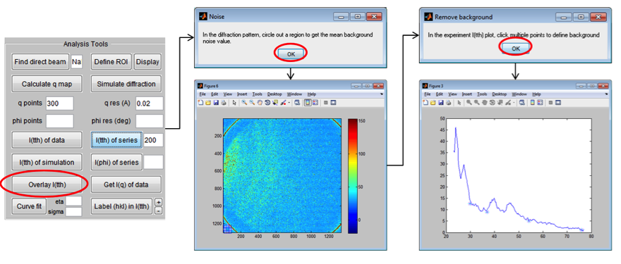
Figure 19: Define noise and background
- Once the background is defined, two windows with diffraction plots will pop up, as Fig. 20. The first plot shows the data and the defined background. The second figure shows the data and simulation in two formats. The left one with noise and background, and the right one without.
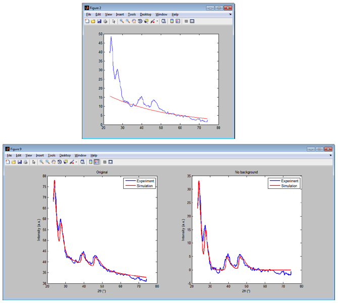
Figure 20: Overlay diffraction data and simulation
- Repeat step (10) if the fitting needs to be improved.
- For two-phase samples, adjust the content of each phase and re-do the simulation to get the best fitting result.
- For some samples with fine grains, the diffraction peaks will be largely broadened. To achieve a better curve fitting, the “Curve fit” function could be used. The “eta” and “sigma” parameters to the right of the button need user inputs. It’s assumed that the diffraction peak shape profile, if using monochromatic x-ray, can be described using pseudo-Voigt function, in which eta and sigma are two key parameters. “eta” is a parameter tuning the contribution of Gaussian and Lorentzian broadening in the Voigt function; “sigma” describes the peak width. (details in Appendix). After conducting previous steps of “Overlay I(tth)”, click “Curve fit” button. A message window with instruction will show up. Click “OK” to proceed. The figure with I(tth) curve will appear. Click two points on the figure to narrow down angle range for further fitting. The diffraction peak(s) within this range will be fitted. Double click the second point to confirm. Then another window will pop up, providing two options for curve fitting: one option is to match the maximum intensities of the data and simulation; the second option is to calculate standard deviation between the data and the simulation, and tune the scaling factor in order to minimize the deviation. For a good fitting, these two options yield very similar results.
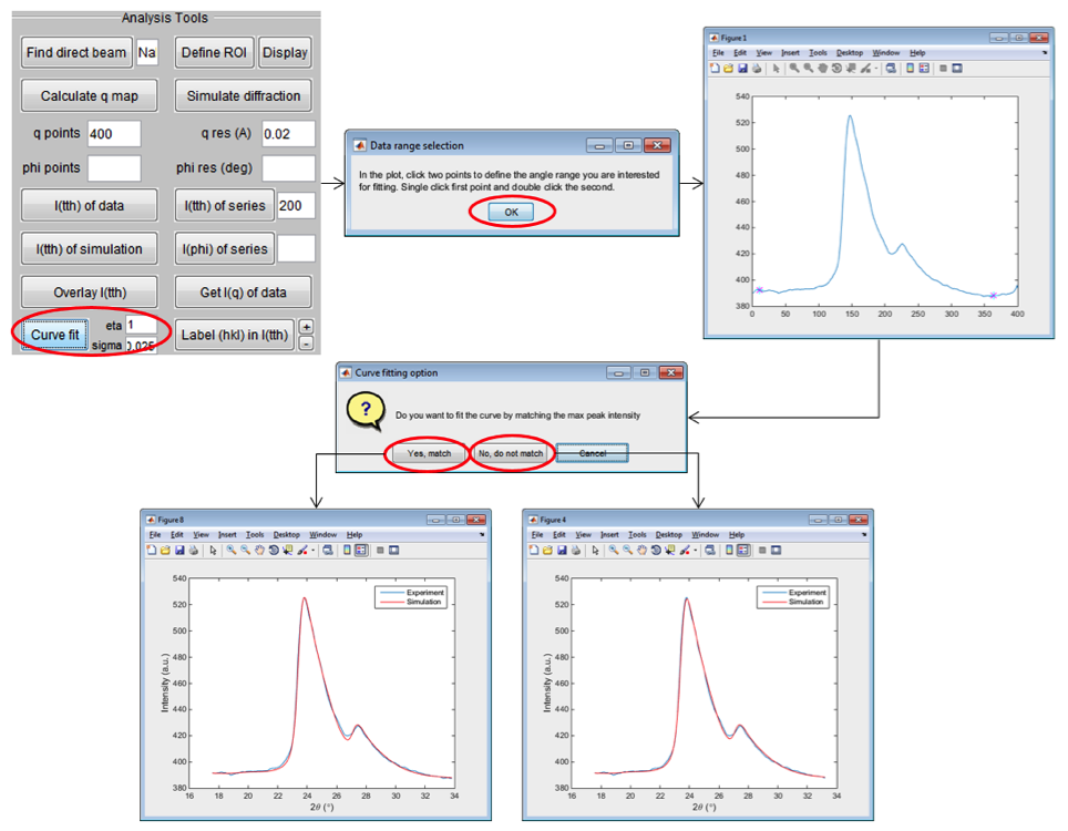
Figure 21: Quantitative curve fitting