Predict diffraction pattern

Prerequisite parameters

• Detector: pixel size, and image pixel dimension
• Sample: crystal structure, lattice parameter, and reference XRD spectrum (i.e. hkl and corresponding diffraction intensity)
• Photon energy spectrum: flux versus energy
• Sample absorption: transmission(%) versus energy. This is only needed when the experiment is in transmission geometry

Adjustable parameters

• Sample-to-detector distance: the shortest distance from the sample to the detector plane (Fig. 3)
• Detector angle: the angle from incident direction to the detector plane surface normal (Fig. 3)
• Direct beam X and Y pixel positions: typically X is negative and Y is positive (Fig. 3)
• Number of harmonic: meaning how many x-ray harmonic energies you’ll consider when simulating “Schematic” diffraction pattern and labeling I(tth) curve
• Scaling factor: meaning n by n image binning when doing data analysis and simulation. n is an integer, i.e. 1, 2, 4 etc. The larger the number, the faster the processing and yet the lower the resolution
• “q points”: number of points in q when calculating I(tth) and I(q)
• “q res (A)”: width or resolution of q when displaying and simulating. The larger this number, the smoother the I(tth) and I(q) plots

Deliverables

• 2D diffraction pattern under the given experiment condition (without noise). The “schematic” pattern show only peak positions with counting the selected harmonic energies, while the “realistic” pattern will consider the entire energy spectrum loaded, reference diffraction intensity, and absorption effect.
• 1D intensity profiles I(tth) and I(q) with all peaks labeled

Procedure for simulating diffraction patterns

1. Input all the known experiment parameters. For repeated simulations, the parameters can be imported from a previously-saved file by clicking the “Load parameters” button.
2. The direct beam X value can be directly input in if the exact position of the detector is known. Otherwise, it may be left blank and the “Find direct beam” function can do the math. Click “Find direct beam” button, and choose “Detector position” in the dialog window popping up, as shown in Fig. 4. Then the direct beam X will be generated. Note that this function only works for the case that the detector position is confined in a circular track with sample facing the center, as shown in the second panel of Fig. 3. Direct beam Y number can be estimated based on the curvature of the diffraction rings in the data. If simulating a diffraction pattern without data, direct beam Y value is typically half of the Image dimension V, i.e. beam is at the center height of the detector.

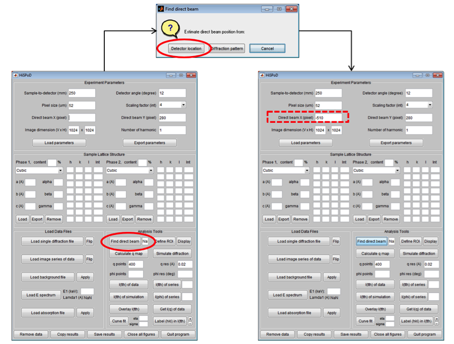
Figure 4: Find direct beam position based on detector position (only for “Circular track” mode)

3. Click “Export parameters” button to save all the numbers in the “Experiment Parameters” module. A typical file saving window will pop up, asking the directory and file name. (Optional)
4. Choose the lattice type from the pull-down menu in the “Sample Lattice Structure” module, and input the lattice parameters and standard diffraction information. For repeated simulations, the parameters can be imported from a previously-saved file by clicking the “Load” button.
5. Input or load the sample information for the secondary phase. (Optional)
6. Input the content of each phase. If there are two phases, the sum of these two numbers should be 100. If both spaces are left blank, the program will take the default value as 50%-50%. (Optional)
7. Click “Remove” button will clear all inputs.
8. Click “Load E spectrum” button to load the energy spectrum. These data files are normally provided to the users by the beamline. Also, users can calculate the energy spectrum using the XOP software for the given undulator type and gap. A message window will then pop up asking the user to circle out multiple peaks (“number of harmonic” that the user filled in) in the spectrum. Click “OK” and the energy spectrum plot will show up. Use mouse to circle the interested and the program will automatically find the peak positions and marked them in the plot. The energy of the first selected harmonic, wavelength, and the name of the loaded file will show up in the GUI control panel, as illustrated in Fig. 5. Note that users don’t have to always select the 1^st harmonic energy, particularly when dealing with small undulator gap and strong absorption samples.

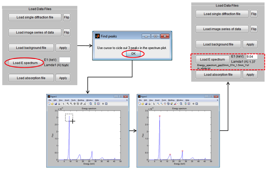
Figure 5: Load energy spectrum and find harmonic energies

9. Click “Load absorption file” button to load x-ray transmission curve. This is needed only for transmission geometry. The x-ray mass attenuation coefficient of elements can be found on the webpage of NIST. The loaded data will then be plotted in a window, as shown in Fig. 6.
10. Click “Apply” button next to the “Load absorption file” button to apply modification of the energy spectrum. A plot window with the original energy spectrum, the transmission curve, and the modified energy spectrum will pop up, together with a message window asking whether to keep the change or select another absorption file. If choose “Yes, keep it”, a window showing only the modified energy spectrum will pop up. Also, the name of the absorption file will appear in the GUI control panel, as shown in Fig. 7. If choose “No, select another file”, then choose another one. Choose “Cancel” if do not want to do anything.

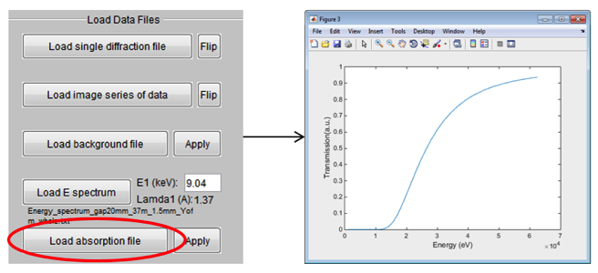
Figure 6: Load absorption file (transmission% vs energy)

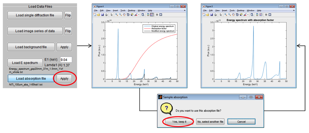
Figure 7: Apply sample absorption to modify the energy spectrum

11. Click “Simulate diffraction” button to calculate the diffraction pattern with the given experiment parameters and sample structure. A dialog window will pop up and provide two options. Click “Schematic” to generate a simple pattern with the diffraction peak position marked. In this mode, only the selected harmonic energies will be considered. Click “Realistic” to simulate a diffraction pattern that resembles more like the true experiment data. In this mode, the reference diffraction intensity of each (hkl), energy spectrum, and absorption from sample and filter will all be considered. After click the “Realistic” button, an input window will pop up, asking for a number range from 0.5 to 3. This is a dummy scaling number, and the larger the number, the more data points from the energy spectrum will be used for simulating, i.e. simulation with higher energy resolution. After inputting a number and clicking “OK”, a message window will pop up with instruction of pointing out the harmonic peak positions. Then, in the energy spectrum plot, single click in the vicinity of each peak (the program will find the true peak position automatically) and double click the last point to confirm selection.

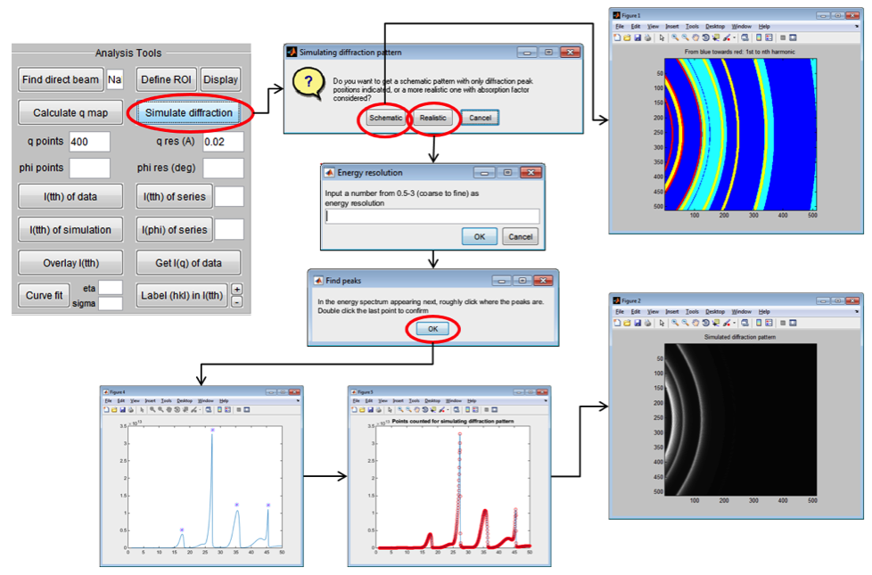
Figure 8: Simulate diffraction pattern

12. In the “Tools” module, input number of points for I(tth) or I(q) and q resolution for getting 1D data. “Points” should be smaller than the number of pixels in the diffraction pattern along horizontal direction. “q res (A)” should be larger than the pixel resolution. Typical q resolution ranges from 0.005 to 0.05.
13. Click “I(tth) of simulation” button to extract the 1D intensity profile, as Fig. 9. In this function, the program will first calculate the q map corresponding to the 1^st harmonic energy, and then average intensities of those pixels that have similar q values. In the end, the program convert I(q) back to I(tth).

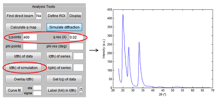
Figure 9: Calculate I(tth) from the simulated diffraction pattern

14. Click “Label (hkl) in I(tth)” button to index the 1D intensity profile. A dialog window will pop up with options to index the experiment data or simulation. Click “Simulation” button, and reference diffraction peaks of the sample will be displayed on I(tth) plot. The color of the line/bar indicates to which harmonic energy a specific peak belongs. Solid line is for phase 1 and dashed line is for phase 2. The relative heights of these reference lines can be adjusted by clicking the “+” and “-” buttons.

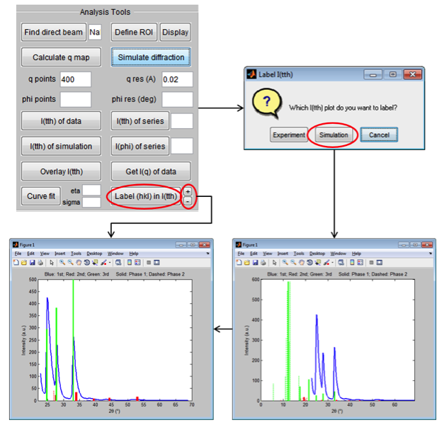
Figure 10: Index peaks on 1D diffraction intensity profile I(tth)